Flow-based policies can model complex, multimodal action distributions that simpler policies cannot. But optimizing a flow policy for reward is difficult: each action is produced by integrating a velocity field through a numerical ODE solver, so improving it for return means differentiating through that entire generation process. Two prior strategies address this, but each comes with a fundamental limitation.
Challenge: The Expressivity–Stability Dilemma
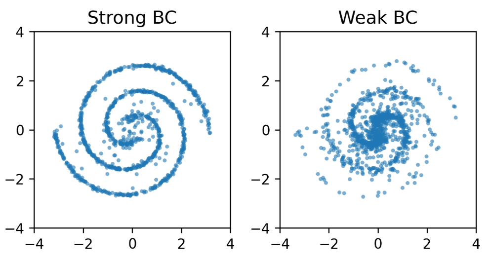
2D Experimentsbehavior under varying BC strength
To see the dilemma concretely, we visualize each method on two 2D synthetic tasks, sweeping the BC regularization strength:
The two synthetic testbeds. Hover a task to highlight its row in the comparison below.
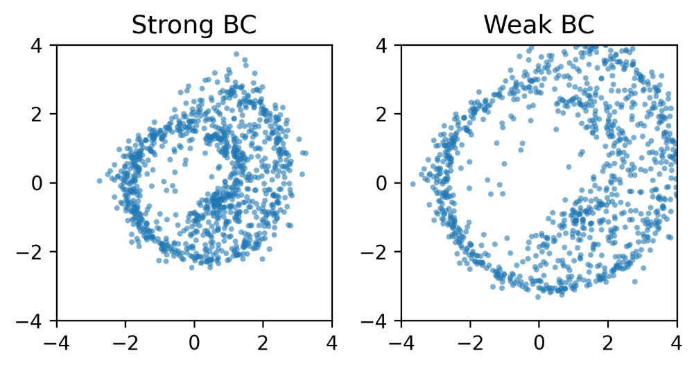
Backprop Through Time (BPTT)
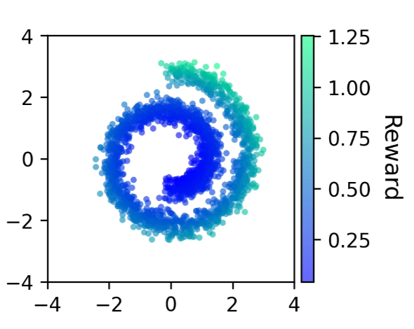
Swiss Roll
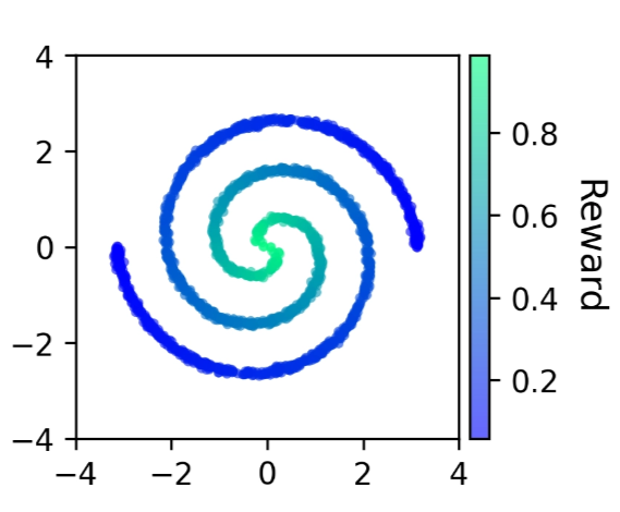
Two Spirals
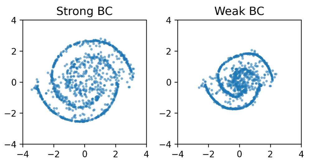
One-step Distillation
Swiss Roll
Two Spirals
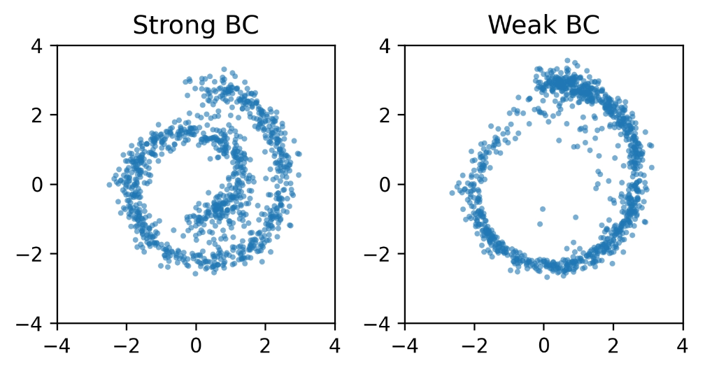
Q-Flow (Ours)
Swiss Roll
Two Spirals
Backprop Through Time (BPTT)
Maximize the critic directly on the action $a \sim \pi_\theta(\cdot \mid s)$ generated by the flow, backpropagating the $Q$-gradient through the entire ODE rollout, with a conditional flow-matching (behavioral-cloning) term anchoring the policy to the data:
$$\mathcal{L}_\pi(\theta) = -\,\mathbb{E}_{\substack{s \sim \mathcal{D} \\ a \sim \pi_\theta(\cdot \mid s)}}\!\bigg[Q_\phi(s, a)\bigg] + \alpha\, \mathbb{E}_{\substack{\tau \sim \mathcal{U}(0,1) \\ x_0 \sim \mathcal{N}(0, I) \\ (s, a) \sim \mathcal{D}}}\!\bigg[\big\|v_\theta(x_\tau, \tau, s) - (a - x_0)\big\|^2\bigg]$$
where $v_\theta$ is the flow's velocity field and $x_\tau = (1-\tau)\,x_0 + \tau\,a$.
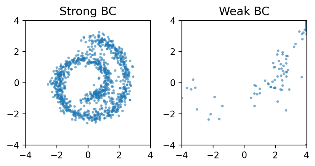
In the 2D experiments above:
Strong BC
Expressive, capturing the complex data structure.
Weak BC
Unstable: backpropagating through the ODE solver destabilizes policy optimization and drifts off the data distribution.
One-step Distillation
FQL2 first fits a behavioral-cloning flow policy $\pi^{\text{BC}}_\theta$, whose velocity field $v_\theta$ is trained by flow matching:
$$\mathcal{L}_{\mathrm{BC}}(\theta) = \mathbb{E}_{\substack{\tau \sim \mathcal{U}(0,1) \\ x_0 \sim \mathcal{N}(0, I) \\ (s, a) \sim \mathcal{D}}}\!\bigg[\big\|v_\theta(x_\tau, \tau, s) - (a - x_0)\big\|^2\bigg]$$
with $x_\tau = (1-\tau)\,x_0 + \tau\,a$.
It then distills this flow into a one-step policy $\pi^{\text{one-step}}_\omega$ that maps noise $x_0$ directly to an action, trained to maximize the critic while staying close to the flow's output (coefficient $\alpha$):
$$\mathcal{L}_\pi(\omega) = -\,\mathbb{E}_{\substack{s \sim \mathcal{D} \\ a^\omega \sim \pi^{\text{one-step}}_\omega(\cdot \mid s)}}\!\bigg[Q_\phi(s, a^\omega)\bigg] + \alpha\, \mathbb{E}_{\substack{s \sim \mathcal{D} \\ a^\omega \sim \pi^{\text{one-step}}_\omega(\cdot \mid s) \\ a^\theta \sim \pi^{\text{BC}}_\theta(\cdot \mid s)}}\!\bigg[\big\|a^\omega - a^\theta\big\|^2\bigg]$$
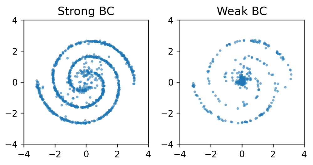
In the 2D experiments above:
Strong BC
Limited Expressivity due to one-step prediction.
Weak BC
Stability gained by avoiding unrolling the solver multiple times.
Q-Flow escapes this trade-off. It keeps the full flow policy yet steers it with the gradient of a learned intermediate value rather than backpropagating through the solver, giving stable optimization at no cost to expressivity. See the method below.